Sampling from and decoding an HMM

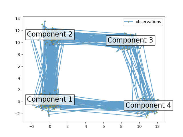
This script shows how to sample points from a Hidden Markov Model (HMM): we use a 4-state model with specified mean and covariance.

The plot shows the sequence of observations generated with the transitions between them. We can see that, as specified by our transition matrix, there are no transition between component 1 and 3.

Then, we decode our model to recover the input parameters.

import numpy as np
import matplotlib.pyplot as plt

from hmmlearn import hmm

# Prepare parameters for a 4-components HMM
# Initial population probability
startprob = np.array([0.6, 0.3, 0.1, 0.0])
# The transition matrix, note that there are no transitions possible
# between component 1 and 3
transmat = np.array([[0.7, 0.2, 0.0, 0.1],
                     [0.3, 0.5, 0.2, 0.0],
                     [0.0, 0.3, 0.5, 0.2],
                     [0.2, 0.0, 0.2, 0.6]])
# The means of each component
means = np.array([[0.0, 0.0],
                  [0.0, 11.0],
                  [9.0, 10.0],
                  [11.0, -1.0]])
# The covariance of each component
covars = .5 * np.tile(np.identity(2), (4, 1, 1))

# Build an HMM instance and set parameters
gen_model = hmm.GaussianHMM(n_components=4, covariance_type="full")

# Instead of fitting it from the data, we directly set the estimated
# parameters, the means and covariance of the components
gen_model.startprob_ = startprob
gen_model.transmat_ = transmat
gen_model.means_ = means
gen_model.covars_ = covars

# Generate samples
X, Z = gen_model.sample(500)

# Plot the sampled data
fig, ax = plt.subplots()
ax.plot(X[:, 0], X[:, 1], ".-", label="observations", ms=6,
        mfc="orange", alpha=0.7)

# Indicate the component numbers
for i, m in enumerate(means):
    ax.text(m[0], m[1], 'Component %i' % (i + 1),
            size=17, horizontalalignment='center',
            bbox=dict(alpha=.7, facecolor='w'))
ax.legend(loc='best')
fig.show()

Now, let’s ensure we can recover our parameters.

scores = list()
models = list()
for n_components in (3, 4, 5):
    for idx in range(10):
        # define our hidden Markov model
        model = hmm.GaussianHMM(n_components=n_components,
                                covariance_type='full',
                                random_state=idx)
        model.fit(X[:X.shape[0] // 2])  # 50/50 train/validate
        models.append(model)
        scores.append(model.score(X[X.shape[0] // 2:]))
        print(f'Converged: {model.monitor_.converged}'
              f'\tScore: {scores[-1]}')

# get the best model
model = models[np.argmax(scores)]
n_states = model.n_components
print(f'The best model had a score of {max(scores)} and {n_states} '
      'states')

# use the Viterbi algorithm to predict the most likely sequence of states
# given the model
states = model.predict(X)

Converged: True Score: -1464.4537093530705
Converged: True Score: -1160.0376561677629
Converged: True Score: -1073.9817948298912
Converged: True Score: -1073.9817948298914
Converged: True Score: -1152.6403059684721
Converged: True Score: -1073.9817948298937
Converged: True Score: -1073.9817948298905
Converged: True Score: -1073.9817948298848
Converged: True Score: -1073.9817945857505
Converged: True Score: -1073.9817948298914
Converged: True Score: -904.4104011027309
Converged: True Score: -1079.9023012348102
Converged: True Score: -932.6769411019295
Converged: True Score: -1074.6321161892483
Converged: True Score: -932.2719797716564
Converged: True Score: -1036.3526634658729
Converged: True Score: -968.3080856410083
Converged: True Score: -932.2719797716553
Converged: True Score: -932.2719797716552
Converged: True Score: -931.5620928935114
Converged: True Score: -1046.6202745712717
Converged: True Score: -1011.721789620891
Converged: True Score: -938.4388006572714
Converged: True Score: -945.9969557801252
Converged: True Score: -939.1979464345783
Converged: True Score: -854.4184482162858
Converged: True Score: -944.7507615355137
Converged: True Score: -937.6419960807413
Converged: True Score: -863.8523113387329
Converged: True Score: -824.9904922608579
The best model had a score of -824.9904922608579 and 5 states

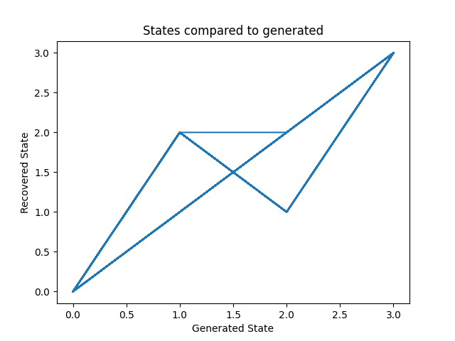
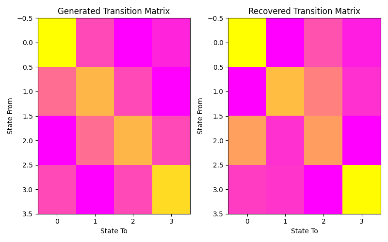
Let’s plot our states compared to those generated and our transition matrix to get a sense of our model. We can see that the recovered states follow the same path as the generated states, just with the identities of the states transposed (i.e. instead of following a square as in the first figure, the nodes are switch around but this does not change the basic pattern). The same is true for the transition matrix.

# plot model states over time
fig, ax = plt.subplots()
ax.plot(Z, states)
ax.set_title('States compared to generated')
ax.set_xlabel('Generated State')
ax.set_ylabel('Recovered State')
fig.show()

# plot the transition matrix
fig, (ax1, ax2) = plt.subplots(1, 2, figsize=(8, 5))
ax1.imshow(gen_model.transmat_, aspect='auto', cmap='spring')
ax1.set_title('Generated Transition Matrix')
ax2.imshow(model.transmat_, aspect='auto', cmap='spring')
ax2.set_title('Recovered Transition Matrix')
for ax in (ax1, ax2):
    ax.set_xlabel('State To')
    ax.set_ylabel('State From')

fig.tight_layout()
fig.show()

• 
•