Dishonest Casino Example

We’ll use the ubiquitous dishonest casino example to demonstrate how to train a Hidden Markov Model (HMM) on somewhat realistic test data (e.g. http://www.mcb111.org/w06/durbin_book.pdf Chapter 3).

In this example, we suspect that a casino is trading out a fair die (singular or dice) for a loaded die. We want to figure out 1) when the loaded die was used (i.e. the most likely path) 2) how often the loaded die is used (i.e. the transition probabilities) and 3) the probabilities for each outcome of a roll for the loaded die (i.e. the emission probabilities).

First, import necessary modules and functions.

import numpy as np
import matplotlib.pyplot as plt

from hmmlearn import hmm

Now, let’s act as the casino and exchange a fair die for a loaded one and generate a series of rolls that someone at the casino would observe.

# make our generative model with two components, a fair die and a
# loaded die
gen_model = hmm.CategoricalHMM(n_components=2, random_state=99)

# the first state is the fair die so let's start there so no one
# catches on right away
gen_model.startprob_ = np.array([1.0, 0.0])

# now let's say that we sneak the loaded die in:
# here, we have a 95% chance to continue using the fair die and a 5%
# chance to switch to the loaded die
# when we enter the loaded die state, we have a 90% chance of staying
# in that state and a 10% chance of leaving
gen_model.transmat_ = np.array([[0.95, 0.05],
                                [0.1, 0.9]])

# now let's set the emission means:
# the first state is a fair die with equal probabilities and the
# second is loaded by being biased toward rolling a six
gen_model.emissionprob_ = \
    np.array([[1 / 6, 1 / 6, 1 / 6, 1 / 6, 1 / 6, 1 / 6],
              [1 / 10, 1 / 10, 1 / 10, 1 / 10, 1 / 10, 1 / 2]])

# simulate the loaded dice rolls
rolls, gen_states = gen_model.sample(30000)

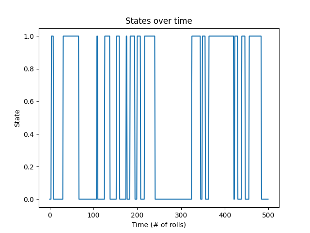
# plot states over time, let's just look at the first rolls for clarity
fig, ax = plt.subplots()
ax.plot(gen_states[:500])
ax.set_title('States over time')
ax.set_xlabel('Time (# of rolls)')
ax.set_ylabel('State')
fig.show()

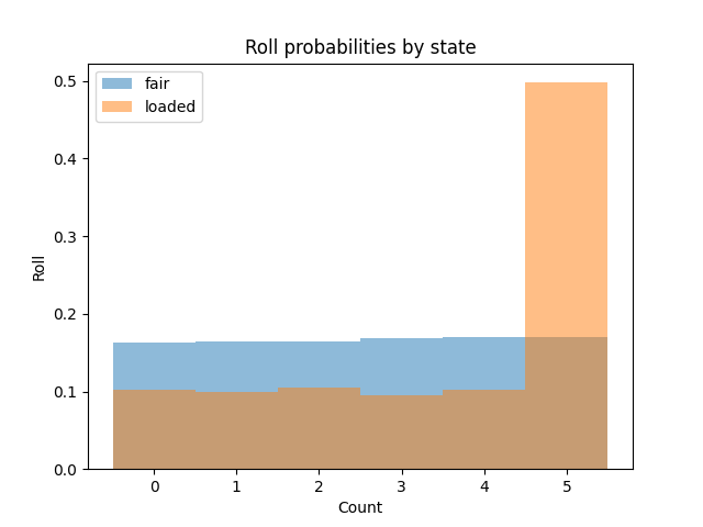
# plot rolls for the fair and loaded states
fig, ax = plt.subplots()
ax.hist(rolls[gen_states == 0], label='fair', alpha=0.5,
        bins=np.arange(7) - 0.5, density=True)
ax.hist(rolls[gen_states == 1], label='loaded', alpha=0.5,
        bins=np.arange(7) - 0.5, density=True)
ax.set_title('Roll probabilities by state')
ax.set_xlabel('Count')
ax.set_ylabel('Roll')
ax.legend()
fig.show()

• 
• 

Now, let’s see if we can recover our hidden states, transmission matrix and emission probabilities.

# split our data into training and validation sets (50/50 split)
X_train = rolls[:rolls.shape[0] // 2]
X_validate = rolls[rolls.shape[0] // 2:]

# check optimal score
gen_score = gen_model.score(X_validate)

best_score = best_model = None
n_fits = 50
np.random.seed(13)
for idx in range(n_fits):
    model = hmm.CategoricalHMM(
        n_components=2, random_state=idx,
        init_params='se')  # don't init transition, set it below
    # we need to initialize with random transition matrix probabilities
    # because the default is an even likelihood transition
    # we know transitions are rare (otherwise the casino would get caught!)
    # so let's have an Dirichlet random prior with an alpha value of
    # (0.1, 0.9) to enforce our assumption transitions happen roughly 10%
    # of the time
    model.transmat_ = np.array([np.random.dirichlet([0.9, 0.1]),
                                np.random.dirichlet([0.1, 0.9])])
    model.fit(X_train)
    score = model.score(X_validate)
    print(f'Model #{idx}\tScore: {score}')
    if best_score is None or score > best_score:
        best_model = model
        best_score = score

print(f'Generated score: {gen_score}\nBest score:      {best_score}')

# use the Viterbi algorithm to predict the most likely sequence of states
# given the model
states = best_model.predict(rolls)

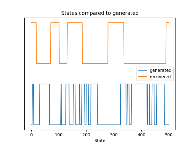
# plot our recovered states compared to generated (aim 1)
fig, ax = plt.subplots()
ax.plot(gen_states[:500], label='generated')
ax.plot(states[:500] + 1.5, label='recovered')
ax.set_yticks([])
ax.set_title('States compared to generated')
ax.set_xlabel('Time (# rolls)')
ax.set_xlabel('State')
ax.legend()
fig.show()

Model #0        Score: -26391.36633375613
Model #1        Score: -26395.55036935765
Model #2        Score: -26405.242643523045
Model #3        Score: -26396.29028373507
Model #4        Score: -26395.550365729432
Model #5        Score: -26375.751287787032
Model #6        Score: -26395.484471121286
Model #7        Score: -26300.67439814206
Model #8        Score: -26265.231791843864
Model #9        Score: -26395.55035772545
Model #10       Score: -26317.463400780533
Model #11       Score: -26405.406087293268
Model #12       Score: -26254.55767639266
Model #13       Score: -26395.48203896293
Model #14       Score: -26247.853013164273
Model #15       Score: -26280.573611463944
Model #16       Score: -26236.969346753132
Model #17       Score: -26320.854926121257
Model #18       Score: -26273.8924196638
Model #19       Score: -26404.09350827867
Model #20       Score: -26405.639243740035
Model #21       Score: -26385.763376940842
Model #22       Score: -26395.4853914974
Model #23       Score: -26395.550366095962
Model #24       Score: -26308.42788082069
Model #25       Score: -26395.506893588612
Model #26       Score: -26296.282415125286
Model #27       Score: -26382.710657722822
Model #28       Score: -26393.754915640107
Model #29       Score: -26396.288808293848
Model #30       Score: -26297.051813976057
Model #31       Score: -26282.173855805813
Model #32       Score: -26315.983239193436
Model #33       Score: -26255.807453160553
Model #34       Score: -26309.540391455714
Model #35       Score: -26395.55036583467
Model #36       Score: -26253.06096935433
Model #37       Score: -26395.550513487622
Model #38       Score: -26395.482877957187
Model #39       Score: -26276.494699725077
Model #40       Score: -26395.55036572371
Model #41       Score: -26395.481806494958
Model #42       Score: -26257.756941739146
Model #43       Score: -26395.55037434898
Model #44       Score: -26282.349594631876
Model #45       Score: -26262.65215987983
Model #46       Score: -26344.068605664717
Model #47       Score: -26229.22005032469
Model #48       Score: -26392.686013999988
Model #49       Score: -26336.186925110036
Generated score: -26230.575868403906
Best score:      -26229.22005032469

Let’s check our learned transition probabilities and see if they match.

print(f'Transmission Matrix Generated:\n{gen_model.transmat_.round(3)}\n\n'
      f'Transmission Matrix Recovered:\n{best_model.transmat_.round(3)}\n\n')

Transmission Matrix Generated:
[[0.95 0.05]
 [0.1  0.9 ]]

Transmission Matrix Recovered:
[[0.922 0.078]
 [0.059 0.941]]

Finally, let’s see if we can tell how the die is loaded.

print(f'Emission Matrix Generated:\n{gen_model.emissionprob_.round(3)}\n\n'
      f'Emission Matrix Recovered:\n{best_model.emissionprob_.round(3)}\n\n')

Emission Matrix Generated:
[[0.167 0.167 0.167 0.167 0.167 0.167]
 [0.1   0.1   0.1   0.1   0.1   0.5  ]]

Emission Matrix Recovered:
[[0.106 0.108 0.114 0.105 0.113 0.454]
 [0.168 0.168 0.167 0.171 0.172 0.153]]

In this case, we were able to get very good estimates of the transition and emission matrices, but decoding the states was imperfect. That’s because the decoding algorithm is greedy and picks the most likely series of states which isn’t necessarily what happens in real life. Even so, our model could tell us when to watch for the loaded die and we’d have a better chance at catching them red-handed.