Note
Go to the end to download the full example code.
Learning an HMM using VI and EM over a set of Gaussian sequences#
We train models with a variety of number of states (N) for each algorithm, and then examine which model is “best”, by printing the log-likelihood or variational lower bound for each N. We will see that an HMM trained using VI will prefer the correct number of states, while an HMM learning with EM will prefer as many states as possible. Note, for models trained with EM, some other criteria such as AIC/BIC, or held out test data, could be used to select the correct number of hidden states.
Training VI(1) Variational Lower Bound=-528.5243461575363 Iterations=3
Training EM(1) Final Log Likelihood=-978.1330363616133 Iterations=3
Training VI(1) Variational Lower Bound=-528.5243461575363 Iterations=3
Training EM(1) Final Log Likelihood=-978.1330363616133 Iterations=3
Training VI(1) Variational Lower Bound=-528.5243461575363 Iterations=3
Training EM(1) Final Log Likelihood=-978.1330363616133 Iterations=3
Training VI(1) Variational Lower Bound=-528.5243461575363 Iterations=3
Training EM(1) Final Log Likelihood=-978.1330363616133 Iterations=3
Training VI(1) Variational Lower Bound=-528.5243461575363 Iterations=3
Training EM(1) Final Log Likelihood=-978.1330363616133 Iterations=3
Training VI(2) Variational Lower Bound=-484.39874601460326 Iterations=26
Training EM(2) Final Log Likelihood=-882.4310706188173 Iterations=26
Training VI(2) Variational Lower Bound=-532.8964116623157 Iterations=17
Training EM(2) Final Log Likelihood=-918.9148210308067 Iterations=17
Training VI(2) Variational Lower Bound=-486.09498533395697 Iterations=45
Training EM(2) Final Log Likelihood=-918.9148216139121 Iterations=45
Training VI(2) Variational Lower Bound=-486.0949851808679 Iterations=56
Training EM(2) Final Log Likelihood=-918.9148211575098 Iterations=56
Training VI(2) Variational Lower Bound=-466.26523178115997 Iterations=20
Training EM(2) Final Log Likelihood=-918.9148218511988 Iterations=20
Training VI(3) Variational Lower Bound=-491.36604396757275 Iterations=70
Training EM(3) Final Log Likelihood=-779.6200734256223 Iterations=70
Training VI(3) Variational Lower Bound=-502.5016699404031 Iterations=93
Model is not converging. Current: -776.3768264355314 is not greater than -776.3768207154641. Delta is -5.720067292713793e-06
Training EM(3) Final Log Likelihood=-776.3768264355314 Iterations=93
Training VI(3) Variational Lower Bound=-503.04395520944945 Iterations=311
Training EM(3) Final Log Likelihood=-776.3769229628026 Iterations=311
Training VI(3) Variational Lower Bound=-534.7503391502202 Iterations=10
Model is not converging. Current: -776.3768247925352 is not greater than -776.376821548232. Delta is -3.244303229621437e-06
Training EM(3) Final Log Likelihood=-776.3768247925352 Iterations=10
Training VI(3) Variational Lower Bound=-471.3061935426669 Iterations=55
Training EM(3) Final Log Likelihood=-916.4417378644604 Iterations=55
Training VI(4) Variational Lower Bound=-540.7416729073641 Iterations=31
Training EM(4) Final Log Likelihood=-769.7551074618457 Iterations=31
Training VI(4) Variational Lower Bound=-515.8069042350241 Iterations=47
Training EM(4) Final Log Likelihood=-769.7550669902676 Iterations=47
Training VI(4) Variational Lower Bound=-494.4704787498257 Iterations=51
Training EM(4) Final Log Likelihood=-795.0238974815446 Iterations=51
Training VI(4) Variational Lower Bound=-494.47047905956845 Iterations=72
Training EM(4) Final Log Likelihood=-771.8693209666542 Iterations=72
Training VI(4) Variational Lower Bound=-439.4628675570252 Iterations=89
Training EM(4) Final Log Likelihood=-769.7551006939436 Iterations=89
Training VI(5) Variational Lower Bound=-536.6280931208877 Iterations=8
Training EM(5) Final Log Likelihood=-649.9020096429672 Iterations=8
Training VI(5) Variational Lower Bound=-536.628093120888 Iterations=11
Training EM(5) Final Log Likelihood=-757.1294446680433 Iterations=11
Training VI(5) Variational Lower Bound=-515.9488121505126 Iterations=90
Training EM(5) Final Log Likelihood=-651.3404017551702 Iterations=90
Training VI(5) Variational Lower Bound=-532.4614280318912 Iterations=70
Training EM(5) Final Log Likelihood=-649.898839819312 Iterations=70
Training VI(5) Variational Lower Bound=-517.8642877403857 Iterations=84
Training EM(5) Final Log Likelihood=-653.0093918227705 Iterations=84
Training VI(6) Variational Lower Bound=-530.7099205460099 Iterations=209
Training EM(6) Final Log Likelihood=-638.2879478022887 Iterations=209
Training VI(6) Variational Lower Bound=-515.547978366197 Iterations=119
Training EM(6) Final Log Likelihood=-642.8154476766686 Iterations=119
Training VI(6) Variational Lower Bound=-532.6891221970648 Iterations=110
Training EM(6) Final Log Likelihood=-637.1697246409943 Iterations=110
Training VI(6) Variational Lower Bound=-529.5730278013729 Iterations=226
Training EM(6) Final Log Likelihood=-783.2105626544517 Iterations=226
Training VI(6) Variational Lower Bound=-512.2182825398047 Iterations=67
Training EM(6) Final Log Likelihood=-646.0622841873077 Iterations=67
VI(1): -528.5243
VI(2): -466.2652
VI(3): -471.3062
VI(4): -439.4629* <- Best Model
VI(5): -515.9488
VI(6): -512.2183
Best Model VI
[[0.002 0.180 0.517 0.301]
[0.539 0.176 0.002 0.283]
[0.002 0.355 0.443 0.200]
[0.577 0.219 0.002 0.202]]
[[2.320]
[-0.026]
[2.123]
[-1.460]]
[[[0.677]]
[[0.057]]
[[0.793]]
[[0.096]]]
EM(1): -978.1330
EM(2): -882.4311
EM(3): -776.3768
EM(4): -769.7551
EM(5): -649.8988
EM(6): -637.1697* <- Best Model
Best Model EM
[[0.197 0.001 0.257 0.063 0.318 0.164]
[0.418 0.000 0.254 0.158 0.170 0.000]
[0.249 0.189 0.000 0.000 0.239 0.323]
[0.317 0.103 0.000 0.138 0.442 0.000]
[0.352 0.001 0.278 0.000 0.189 0.180]
[0.193 0.000 0.335 0.353 0.119 0.000]]
[[3.020]
[-1.563]
[-1.460]
[1.470]
[-0.023]
[1.482]]
[[[0.052]]
[[0.018]]
[[0.060]]
[[0.046]]
[[0.055]]
[[0.056]]]
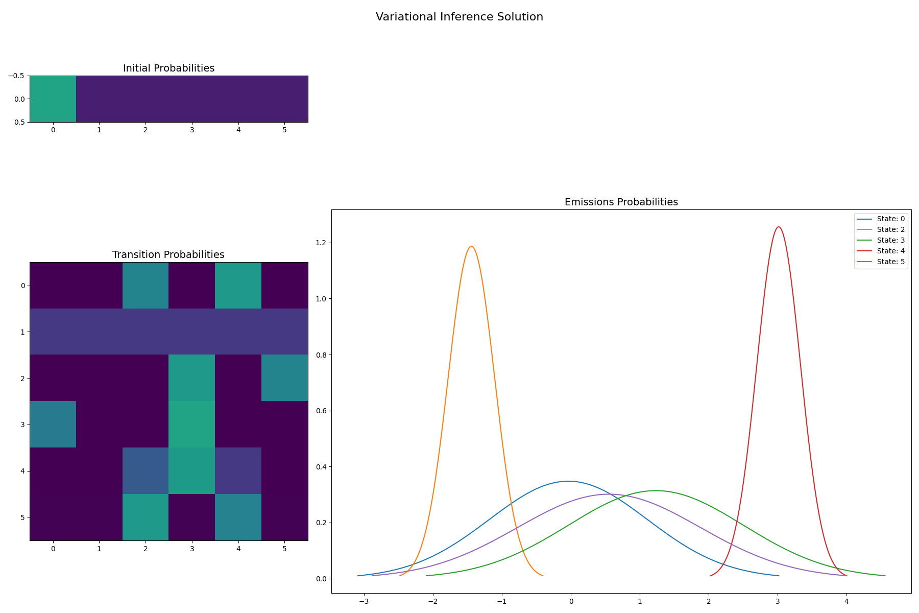
VI solution for 6 states: Notice sparsity among states 1 and 4
[[0.002 0.002 0.451 0.002 0.542 0.002]
[0.167 0.167 0.167 0.167 0.167 0.167]
[0.002 0.002 0.002 0.540 0.002 0.452]
[0.413 0.001 0.001 0.583 0.001 0.001]
[0.002 0.002 0.284 0.546 0.164 0.002]
[0.004 0.004 0.541 0.004 0.442 0.004]]
[[-0.036]
[0.788]
[-1.442]
[1.233]
[3.015]
[0.554]]
[[[1.316]]
[[0.001]]
[[0.113]]
[[1.613]]
[[0.101]]
[[1.753]]]
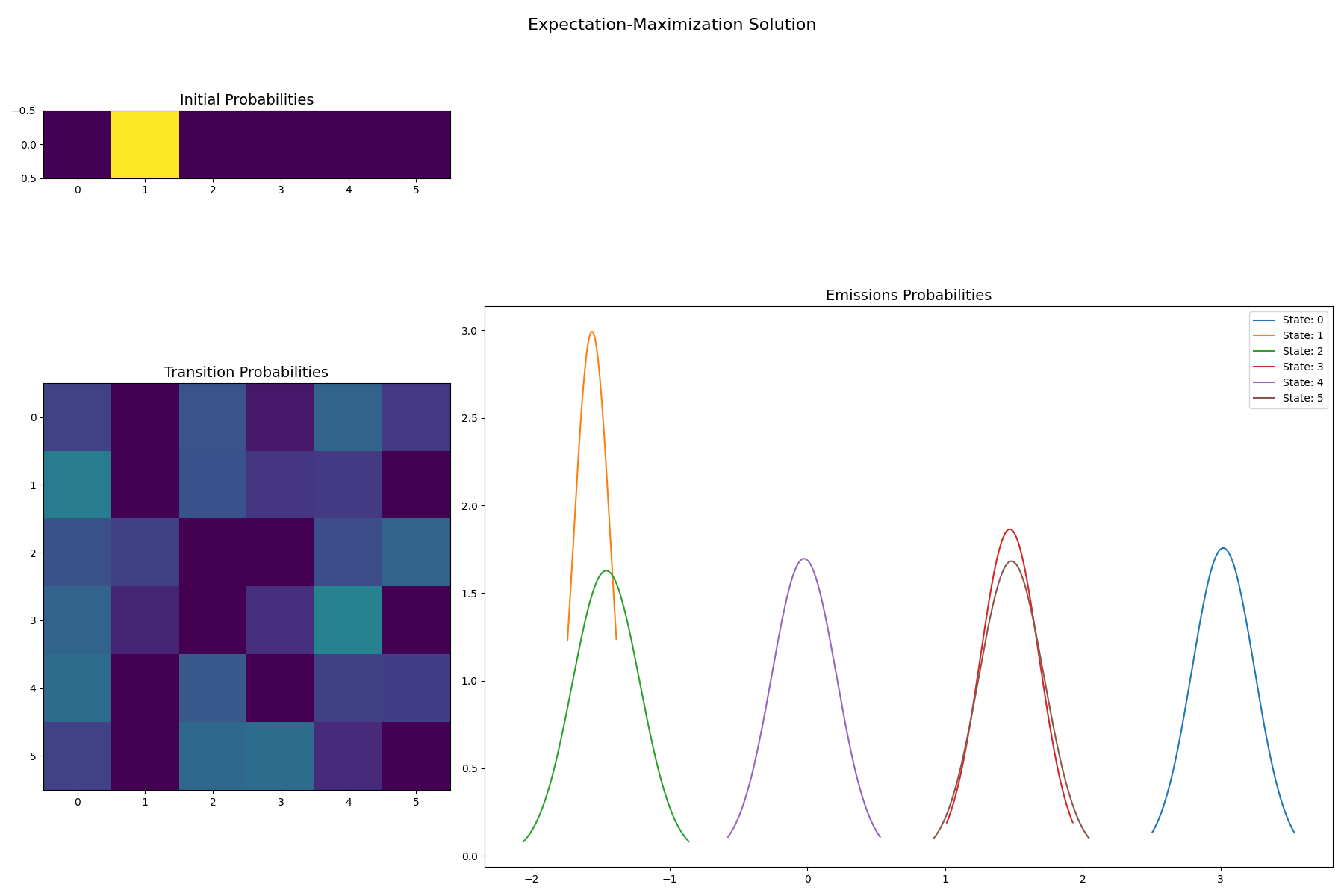
EM solution for 6 states
[[0.197 0.001 0.257 0.063 0.318 0.164]
[0.418 0.000 0.254 0.158 0.170 0.000]
[0.249 0.189 0.000 0.000 0.239 0.323]
[0.317 0.103 0.000 0.138 0.442 0.000]
[0.352 0.001 0.278 0.000 0.189 0.180]
[0.193 0.000 0.335 0.353 0.119 0.000]]
[[3.020]
[-1.563]
[-1.460]
[1.470]
[-0.023]
[1.482]]
[[[0.052]]
[[0.018]]
[[0.060]]
[[0.046]]
[[0.055]]
[[0.056]]]
import collections
import numpy as np
import matplotlib.pyplot as plt
import matplotlib.gridspec as gs
import scipy.stats

from sklearn.utils import check_random_state

from hmmlearn import hmm, vhmm
import matplotlib


def gaussian_hinton_diagram(startprob, transmat, means,
                            variances, vmin=0, vmax=1, infer_hidden=True):
    """
    Show the initial state probabilities, the transition probabilities
    as heatmaps, and draw the emission distributions.
    """

    num_states = transmat.shape[0]

    f = plt.figure(figsize=(3*(num_states), 2*num_states))
    grid = gs.GridSpec(3, 3)

    ax = f.add_subplot(grid[0, 0])
    ax.imshow(startprob[None, :], vmin=vmin, vmax=vmax)
    ax.set_title("Initial Probabilities", size=14)

    ax = f.add_subplot(grid[1:, 0])
    ax.imshow(transmat, vmin=vmin, vmax=vmax)
    ax.set_title("Transition Probabilities", size=14)

    ax = f.add_subplot(grid[1:, 1:])
    for i in range(num_states):
        keep = True
        if infer_hidden:
            if np.all(np.abs(transmat[i] - transmat[i][0]) < 1e-4):
                keep = False
        if keep:
            s_min = means[i] - 10 * variances[i]
            s_max = means[i] + 10 * variances[i]
            xx = np.arange(s_min, s_max, (s_max - s_min) / 1000)
            norm = scipy.stats.norm(means[i], np.sqrt(variances[i]))
            yy = norm.pdf(xx)
            keep = yy > .01
            ax.plot(xx[keep], yy[keep], label="State: {}".format(i))
    ax.set_title("Emissions Probabilities", size=14)
    ax.legend(loc="best")
    f.tight_layout()
    return f

np.set_printoptions(formatter={'float_kind': "{:.3f}".format})
rs = check_random_state(2022)
sample_length = 500
num_samples = 1
# With random initialization, it takes a few tries to find the
# best solution
num_inits = 5
num_states = np.arange(1, 7)
verbose = False


# Prepare parameters for a 4-components HMM
# And Sample several sequences from this model
model = hmm.GaussianHMM(4, init_params="")
model.n_features = 4
# Initial population probability
model.startprob_ = np.array([0.25, 0.25, 0.25, 0.25])
# The transition matrix, note that there are no transitions possible
# between component 1 and 3
model.transmat_ = np.array([[0.2, 0.2, 0.3, 0.3],
                            [0.3, 0.2, 0.2, 0.3],
                            [0.2, 0.3, 0.3, 0.2],
                            [0.3, 0.3, 0.2, 0.2]])
# The means and covariance of each component
model.means_ = np.array([[-1.5],
                         [0],
                         [1.5],
                         [3.]])
model.covars_ = np.array([[0.25],
                          [0.25],
                          [0.25],
                          [0.25]])**2

# Generate training data
sequences = []
lengths = []

for i in range(num_samples):
    sequences.extend(model.sample(sample_length, random_state=rs)[0])
    lengths.append(sample_length)
sequences = np.asarray(sequences)

# Train a suite of models, and keep track of the best model for each
# number of states, and algorithm
best_scores = collections.defaultdict(dict)
best_models = collections.defaultdict(dict)
for n in num_states:
    for i in range(num_inits):
        vi = vhmm.VariationalGaussianHMM(n,
                                         n_iter=1000,
                                         covariance_type="full",
                                         implementation="scaling",
                                         tol=1e-6,
                                         random_state=rs,
                                         verbose=verbose)
        vi.fit(sequences, lengths)
        lb = vi.monitor_.history[-1]
        print(f"Training VI({n}) Variational Lower Bound={lb} "
              f"Iterations={len(vi.monitor_.history)} ")
        if best_models["VI"].get(n) is None or best_scores["VI"][n] < lb:
            best_models["VI"][n] = vi
            best_scores["VI"][n] = lb

        em = hmm.GaussianHMM(n,
                             n_iter=1000,
                             covariance_type="full",
                             implementation="scaling",
                             tol=1e-6,
                             random_state=rs,
                             verbose=verbose)
        em.fit(sequences, lengths)
        ll = em.monitor_.history[-1]
        print(f"Training EM({n}) Final Log Likelihood={ll} "
              f"Iterations={len(vi.monitor_.history)} ")
        if best_models["EM"].get(n) is None or best_scores["EM"][n] < ll:
            best_models["EM"][n] = em
            best_scores["EM"][n] = ll

# Display the model likelihood/variational lower bound for each N
# and show the best learned model
for algo, scores in best_scores.items():
    best = max(scores.values())
    best_n, best_score = max(scores.items(), key=lambda x: x[1])
    for n, score in scores.items():
        flag = "* <- Best Model" if score == best_score else ""
        print(f"{algo}({n}): {score:.4f}{flag}")

    print(f"Best Model {algo}")
    best_model = best_models[algo][best_n]
    print(best_model.transmat_)
    print(best_model.means_)
    print(best_model.covars_)

# Also inpsect the VI model with 6 states, to see how it has sparse structure
vi_model = best_models["VI"][6]
em_model = best_models["EM"][6]
print("VI solution for 6 states: Notice sparsity among states 1 and 4")
print(vi_model.transmat_)
print(vi_model.means_)
print(vi_model.covars_)
print("EM solution for 6 states")
print(em_model.transmat_)
print(em_model.means_)
print(em_model.covars_)

f = gaussian_hinton_diagram(
    vi_model.startprob_,
    vi_model.transmat_,
    vi_model.means_.ravel(),
    vi_model.covars_.ravel(),
)
f.suptitle("Variational Inference Solution", size=16)
f = gaussian_hinton_diagram(
    em_model.startprob_,
    em_model.transmat_,
    em_model.means_.ravel(),
    em_model.covars_.ravel(),
)
f.suptitle("Expectation-Maximization Solution", size=16)

plt.show()
Total running time of the script: (0 minutes 18.045 seconds)