Sampling from and decoding an HMM

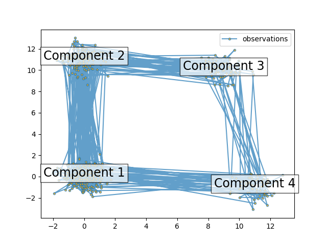
This script shows how to sample points from a Hidden Markov Model (HMM): we use a 4-state model with specified mean and covariance.

The plot shows the sequence of observations generated with the transitions between them. We can see that, as specified by our transition matrix, there are no transition between component 1 and 3.

Then, we decode our model to recover the input parameters.

import numpy as np
import matplotlib.pyplot as plt

from hmmlearn import hmm

# Prepare parameters for a 4-components HMM
# Initial population probability
startprob = np.array([0.6, 0.3, 0.1, 0.0])
# The transition matrix, note that there are no transitions possible
# between component 1 and 3
transmat = np.array([[0.7, 0.2, 0.0, 0.1],
                     [0.3, 0.5, 0.2, 0.0],
                     [0.0, 0.3, 0.5, 0.2],
                     [0.2, 0.0, 0.2, 0.6]])
# The means of each component
means = np.array([[0.0, 0.0],
                  [0.0, 11.0],
                  [9.0, 10.0],
                  [11.0, -1.0]])
# The covariance of each component
covars = .5 * np.tile(np.identity(2), (4, 1, 1))

# Build an HMM instance and set parameters
gen_model = hmm.GaussianHMM(n_components=4, covariance_type="full")

# Instead of fitting it from the data, we directly set the estimated
# parameters, the means and covariance of the components
gen_model.startprob_ = startprob
gen_model.transmat_ = transmat
gen_model.means_ = means
gen_model.covars_ = covars

# Generate samples
X, Z = gen_model.sample(500)

# Plot the sampled data
fig, ax = plt.subplots()
ax.plot(X[:, 0], X[:, 1], ".-", label="observations", ms=6,
        mfc="orange", alpha=0.7)

# Indicate the component numbers
for i, m in enumerate(means):
    ax.text(m[0], m[1], 'Component %i' % (i + 1),
            size=17, horizontalalignment='center',
            bbox=dict(alpha=.7, facecolor='w'))
ax.legend(loc='best')
fig.show()

Now, let’s ensure we can recover our parameters.

scores = list()
models = list()
for n_components in (3, 4, 5):
    for idx in range(10):
        # define our hidden Markov model
        model = hmm.GaussianHMM(n_components=n_components,
                                covariance_type='full',
                                random_state=idx)
        model.fit(X[:X.shape[0] // 2])  # 50/50 train/validate
        models.append(model)
        scores.append(model.score(X[X.shape[0] // 2:]))
        print(f'Converged: {model.monitor_.converged}'
              f'\tScore: {scores[-1]}')

# get the best model
model = models[np.argmax(scores)]
n_states = model.n_components
print(f'The best model had a score of {max(scores)} and {n_states} '
      'states')

# use the Viterbi algorithm to predict the most likely sequence of states
# given the model
states = model.predict(X)

Converged: True Score: -1196.6734103747965
Converged: True Score: -1148.0223169911258
Converged: True Score: -936.6205720650934
Converged: True Score: -936.6205720650966
Converged: True Score: -1179.0274153530877
Converged: True Score: -936.6205720650984
Converged: True Score: -936.6205720650952
Converged: True Score: -936.6205720650984
Converged: True Score: -936.6205720650983
Converged: True Score: -936.6205720650955
Converged: True Score: -865.8165165299154
Converged: True Score: -1013.6977314896502
Converged: True Score: -897.1797465794805
Converged: True Score: -956.8327593258822
Converged: True Score: -865.816516529917
Converged: True Score: -1147.9195638683987
Converged: True Score: -895.329419045251
Converged: True Score: -865.8165165299168
Converged: True Score: -865.8165165299185
Converged: True Score: -817.3266948565933
Converged: True Score: -889.8220050450717
Converged: True Score: -1260.4731144680686
Converged: True Score: -992.7879754718065
Converged: True Score: -1031.882532087015
Converged: True Score: -909.6607906625865
Converged: True Score: -1035.6440752146505
Converged: True Score: -868.7259593506282
Converged: True Score: -966.7484712523376
Converged: True Score: -972.0063169843962
Converged: True Score: -934.6624488533251
The best model had a score of -817.3266948565933 and 4 states

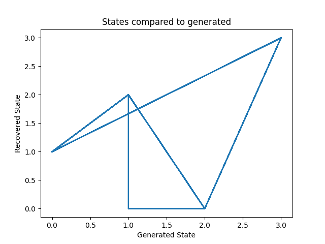
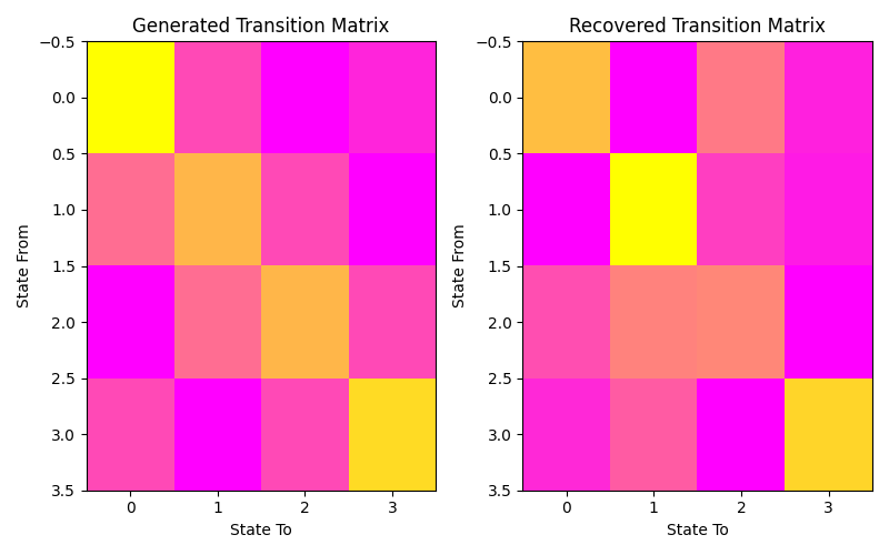
Let’s plot our states compared to those generated and our transition matrix to get a sense of our model. We can see that the recovered states follow the same path as the generated states, just with the identities of the states transposed (i.e. instead of following a square as in the first figure, the nodes are switch around but this does not change the basic pattern). The same is true for the transition matrix.

# plot model states over time
fig, ax = plt.subplots()
ax.plot(Z, states)
ax.set_title('States compared to generated')
ax.set_xlabel('Generated State')
ax.set_ylabel('Recovered State')
fig.show()

# plot the transition matrix
fig, (ax1, ax2) = plt.subplots(1, 2, figsize=(8, 5))
ax1.imshow(gen_model.transmat_, aspect='auto', cmap='spring')
ax1.set_title('Generated Transition Matrix')
ax2.imshow(model.transmat_, aspect='auto', cmap='spring')
ax2.set_title('Recovered Transition Matrix')
for ax in (ax1, ax2):
    ax.set_xlabel('State To')
    ax.set_ylabel('State From')

fig.tight_layout()
fig.show()

• 
•