Using a Hidden Markov Model with Poisson Emissions to Understand Earthquakes

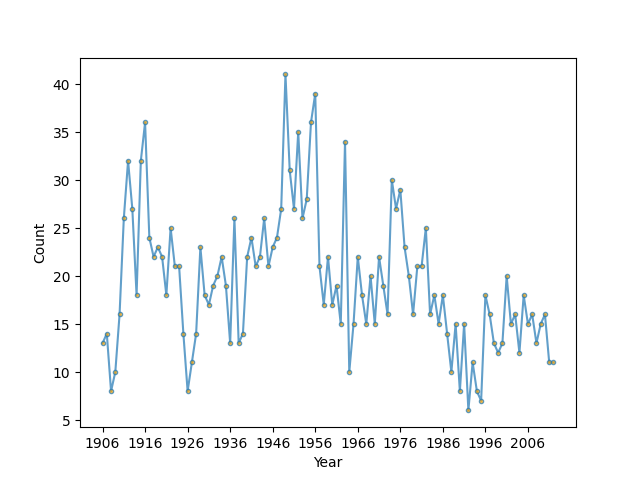
Let’s look at data of magnitude 7+ earthquakes between 1900-2006 in the world collected by the US Geological Survey as described in this textbook: Zucchini & MacDonald, “Hidden Markov Models for Time Series” (https://ayorho.files.wordpress.com/2011/05/chapter1.pdf). The goal is to see if we can separate out different tectonic processes that cause earthquakes based on their frequency of occurance. The idea is that each tectonic boundary may cause earthquakes with a particular distribution of waiting times depending on how active it is. This might tell help us predict future earthquake danger, espeically on a geological time scale.

import numpy as np
import matplotlib.pyplot as plt

from scipy.stats import poisson
from hmmlearn import hmm

# earthquake data from http://earthquake.usgs.gov/
earthquakes = np.array([
    13, 14, 8, 10, 16, 26, 32, 27, 18, 32, 36, 24, 22, 23, 22, 18,
    25, 21, 21, 14, 8, 11, 14, 23, 18, 17, 19, 20, 22, 19, 13, 26,
    13, 14, 22, 24, 21, 22, 26, 21, 23, 24, 27, 41, 31, 27, 35, 26,
    28, 36, 39, 21, 17, 22, 17, 19, 15, 34, 10, 15, 22, 18, 15, 20,
    15, 22, 19, 16, 30, 27, 29, 23, 20, 16, 21, 21, 25, 16, 18, 15,
    18, 14, 10, 15, 8, 15, 6, 11, 8, 7, 18, 16, 13, 12, 13, 20,
    15, 16, 12, 18, 15, 16, 13, 15, 16, 11, 11])


# Plot the sampled data
fig, ax = plt.subplots()
ax.plot(earthquakes, ".-", ms=6, mfc="orange", alpha=0.7)
ax.set_xticks(range(0, earthquakes.size, 10))
ax.set_xticklabels(range(1906, 2007, 10))
ax.set_xlabel('Year')
ax.set_ylabel('Count')
fig.show()

Now, fit a Poisson Hidden Markov Model to the data.

scores = list()
models = list()
for n_components in range(1, 5):
    for idx in range(10):  # ten different random starting states
        # define our hidden Markov model
        model = hmm.PoissonHMM(n_components=n_components, random_state=idx,
                               n_iter=10)
        model.fit(earthquakes[:, None])
        models.append(model)
        scores.append(model.score(earthquakes[:, None]))
        print(f'Converged: {model.monitor_.converged}\t\t'
              f'Score: {scores[-1]}')

# get the best model
model = models[np.argmax(scores)]
print(f'The best model had a score of {max(scores)} and '
      f'{model.n_components} components')

# use the Viterbi algorithm to predict the most likely sequence of states
# given the model
states = model.predict(earthquakes[:, None])

Converged: True         Score: -391.9189281654951
Converged: True         Score: -391.9189281654951
Converged: True         Score: -391.9189281654951
Converged: True         Score: -391.9189281654951
Converged: True         Score: -391.9189281654951
Converged: True         Score: -391.9189281654951
Converged: True         Score: -391.9189281654951
Converged: True         Score: -391.9189281654951
Converged: True         Score: -391.9189281654951
Converged: True         Score: -391.9189281654951
Converged: True         Score: -341.89397049875356
Converged: True         Score: -341.88244772721345
Converged: True         Score: -342.1445482378532
Converged: True         Score: -341.8929674859709
Converged: True         Score: -341.8855538199329
Converged: True         Score: -342.2876227612777
Converged: True         Score: -342.5369292103593
Converged: True         Score: -341.8875020776218
Converged: True         Score: -341.8789363379975
Converged: True         Score: -342.97038817436965
Converged: True         Score: -343.0429169039883
Converged: True         Score: -342.08452039551764
Converged: True         Score: -342.6892743201981
Converged: True         Score: -328.5977427805311
Converged: True         Score: -341.66130011064183
Converged: True         Score: -329.06399427716025
Converged: True         Score: -329.50502535576027
Converged: True         Score: -338.9078699324075
Converged: True         Score: -328.7562782189654
Converged: True         Score: -337.6515744961049
Converged: True         Score: -328.14045680319686
Converged: True         Score: -340.59777383065585
Converged: True         Score: -330.46705382979616
Converged: True         Score: -341.56334292712455
Converged: True         Score: -328.0212654423776
Converged: True         Score: -340.86474747756466
Converged: True         Score: -339.5597855572184
Converged: True         Score: -328.6984713056866
Converged: True         Score: -328.8760462922794
Converged: True         Score: -340.13188775835465
The best model had a score of -328.0212654423776 and 4 components

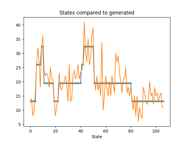
Let’s plot the waiting times from our most likely series of states of earthquake activity with the earthquake data. As we can see, the model with the maximum likelihood had different states which may reflect times of varying earthquake danger.

# plot model states over time
fig, ax = plt.subplots()
ax.plot(model.lambdas_[states], ".-", ms=6, mfc="orange")
ax.plot(earthquakes)
ax.set_title('States compared to generated')
ax.set_xlabel('State')

Text(0.5, 23.52222222222222, 'State')

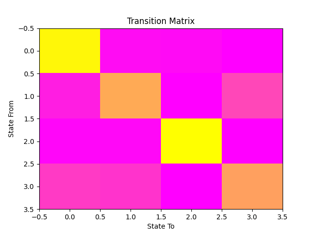
Fortunately, 2006 ended with a period of relative tectonic stability, and, if we look at our transition matrix, we can see that the off-diagonal terms are small, meaning that the state transitions are rare and it’s unlikely that there will be high earthquake danger in the near future.

fig, ax = plt.subplots()
ax.imshow(model.transmat_, aspect='auto', cmap='spring')
ax.set_title('Transition Matrix')
ax.set_xlabel('State To')
ax.set_ylabel('State From')

Text(31.222222222222214, 0.5, 'State From')

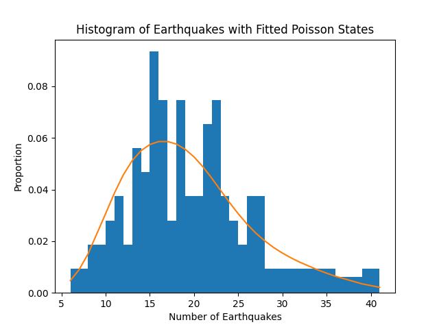
Finally, let’s look at the distribution of earthquakes compared to our waiting time parameter values. We can see that our model fits the distribution fairly well, replicating results from the reference.

# get probabilities for each state given the data, take the average
# to find the proportion of time in that state
prop_per_state = model.predict_proba(earthquakes[:, None]).mean(axis=0)

# earthquake counts to plot
bins = sorted(np.unique(earthquakes))

fig, ax = plt.subplots()
ax.hist(earthquakes, bins=bins, density=True)
ax.plot(bins, poisson.pmf(bins, model.lambdas_).T @ prop_per_state)
ax.set_title('Histogram of Earthquakes with Fitted Poisson States')
ax.set_xlabel('Number of Earthquakes')
ax.set_ylabel('Proportion')

plt.show()