Sampling from and decoding an HMM

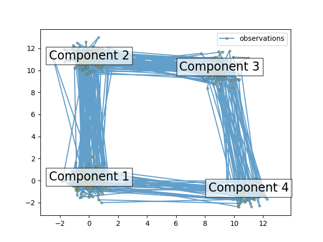
This script shows how to sample points from a Hidden Markov Model (HMM): we use a 4-state model with specified mean and covariance.

The plot shows the sequence of observations generated with the transitions between them. We can see that, as specified by our transition matrix, there are no transition between component 1 and 3.

Then, we decode our model to recover the input parameters.

import numpy as np
import matplotlib.pyplot as plt

from hmmlearn import hmm

# Prepare parameters for a 4-components HMM
# Initial population probability
startprob = np.array([0.6, 0.3, 0.1, 0.0])
# The transition matrix, note that there are no transitions possible
# between component 1 and 3
transmat = np.array([[0.7, 0.2, 0.0, 0.1],
                     [0.3, 0.5, 0.2, 0.0],
                     [0.0, 0.3, 0.5, 0.2],
                     [0.2, 0.0, 0.2, 0.6]])
# The means of each component
means = np.array([[0.0, 0.0],
                  [0.0, 11.0],
                  [9.0, 10.0],
                  [11.0, -1.0]])
# The covariance of each component
covars = .5 * np.tile(np.identity(2), (4, 1, 1))

# Build an HMM instance and set parameters
gen_model = hmm.GaussianHMM(n_components=4, covariance_type="full")

# Instead of fitting it from the data, we directly set the estimated
# parameters, the means and covariance of the components
gen_model.startprob_ = startprob
gen_model.transmat_ = transmat
gen_model.means_ = means
gen_model.covars_ = covars

# Generate samples
X, Z = gen_model.sample(500)

# Plot the sampled data
fig, ax = plt.subplots()
ax.plot(X[:, 0], X[:, 1], ".-", label="observations", ms=6,
        mfc="orange", alpha=0.7)

# Indicate the component numbers
for i, m in enumerate(means):
    ax.text(m[0], m[1], 'Component %i' % (i + 1),
            size=17, horizontalalignment='center',
            bbox=dict(alpha=.7, facecolor='w'))
ax.legend(loc='best')
fig.show()

Now, let’s ensure we can recover our parameters.

scores = list()
models = list()
for n_components in (3, 4, 5):
    for idx in range(10):
        # define our hidden Markov model
        model = hmm.GaussianHMM(n_components=n_components,
                                covariance_type='full',
                                random_state=idx)
        model.fit(X[:X.shape[0] // 2])  # 50/50 train/validate
        models.append(model)
        scores.append(model.score(X[X.shape[0] // 2:]))
        print(f'Converged: {model.monitor_.converged}'
              f'\tScore: {scores[-1]}')

# get the best model
model = models[np.argmax(scores)]
n_states = model.n_components
print(f'The best model had a score of {max(scores)} and {n_states} '
      'states')

# use the Viterbi algorithm to predict the most likely sequence of states
# given the model
states = model.predict(X)

Converged: True Score: -1576.1753905467317
Converged: True Score: -1179.2235368637366
Converged: True Score: -1250.4232852250461
Converged: True Score: -1250.423285225043
Converged: True Score: -1225.1550378569789
Converged: True Score: -1250.4232852250436
Converged: True Score: -1250.4232852250425
Converged: True Score: -1250.4232852250402
Converged: True Score: -1250.423285225039
Converged: True Score: -1250.4232852250395
Converged: True Score: -1135.0399742332147
Converged: True Score: -1078.5651921877454
Converged: True Score: -1209.7488003377325
Converged: True Score: -1343.9580402942222
Converged: True Score: -1123.7381638734348
Converged: True Score: -1223.7070036303828
Converged: True Score: -1197.5094287450333
Converged: True Score: -1121.7247334015203
Converged: True Score: -1117.5244481532716
Converged: True Score: -1117.9925570287362
Converged: True Score: -1264.910201511487
Converged: True Score: -1015.3354311749436
Converged: True Score: -1139.4481688328324
Converged: True Score: -1253.126595190962
Converged: True Score: -1164.0728223476915
Converged: True Score: -1149.9952377598836
Converged: True Score: -1220.4604840715806
Converged: True Score: -1022.4576591442977
Converged: True Score: -1052.616926381614
Converged: True Score: -1128.1136948555557
The best model had a score of -1015.3354311749436 and 5 states

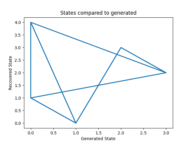
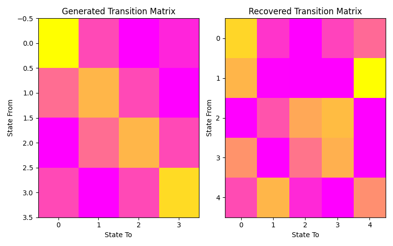
Let’s plot our states compared to those generated and our transition matrix to get a sense of our model. We can see that the recovered states follow the same path as the generated states, just with the identities of the states transposed (i.e. instead of following a square as in the first figure, the nodes are switch around but this does not change the basic pattern). The same is true for the transition matrix.

# plot model states over time
fig, ax = plt.subplots()
ax.plot(Z, states)
ax.set_title('States compared to generated')
ax.set_xlabel('Generated State')
ax.set_ylabel('Recovered State')
fig.show()

# plot the transition matrix
fig, (ax1, ax2) = plt.subplots(1, 2, figsize=(8, 5))
ax1.imshow(gen_model.transmat_, aspect='auto', cmap='spring')
ax1.set_title('Generated Transition Matrix')
ax2.imshow(model.transmat_, aspect='auto', cmap='spring')
ax2.set_title('Recovered Transition Matrix')
for ax in (ax1, ax2):
    ax.set_xlabel('State To')
    ax.set_ylabel('State From')

fig.tight_layout()
fig.show()

• 
•