Sampling from and decoding an HMM

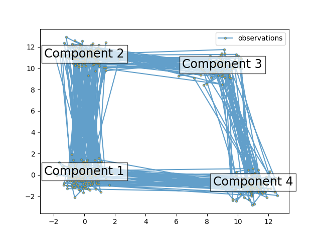
This script shows how to sample points from a Hidden Markov Model (HMM): we use a 4-state model with specified mean and covariance.

The plot shows the sequence of observations generated with the transitions between them. We can see that, as specified by our transition matrix, there are no transition between component 1 and 3.

Then, we decode our model to recover the input parameters.

import numpy as np
import matplotlib.pyplot as plt

from hmmlearn import hmm

# Prepare parameters for a 4-components HMM
# Initial population probability
startprob = np.array([0.6, 0.3, 0.1, 0.0])
# The transition matrix, note that there are no transitions possible
# between component 1 and 3
transmat = np.array([[0.7, 0.2, 0.0, 0.1],
                     [0.3, 0.5, 0.2, 0.0],
                     [0.0, 0.3, 0.5, 0.2],
                     [0.2, 0.0, 0.2, 0.6]])
# The means of each component
means = np.array([[0.0, 0.0],
                  [0.0, 11.0],
                  [9.0, 10.0],
                  [11.0, -1.0]])
# The covariance of each component
covars = .5 * np.tile(np.identity(2), (4, 1, 1))

# Build an HMM instance and set parameters
gen_model = hmm.GaussianHMM(n_components=4, covariance_type="full")

# Instead of fitting it from the data, we directly set the estimated
# parameters, the means and covariance of the components
gen_model.startprob_ = startprob
gen_model.transmat_ = transmat
gen_model.means_ = means
gen_model.covars_ = covars

# Generate samples
X, Z = gen_model.sample(500)

# Plot the sampled data
fig, ax = plt.subplots()
ax.plot(X[:, 0], X[:, 1], ".-", label="observations", ms=6,
        mfc="orange", alpha=0.7)

# Indicate the component numbers
for i, m in enumerate(means):
    ax.text(m[0], m[1], 'Component %i' % (i + 1),
            size=17, horizontalalignment='center',
            bbox=dict(alpha=.7, facecolor='w'))
ax.legend(loc='best')
fig.show()

Now, let’s ensure we can recover our parameters.

scores = list()
models = list()
for n_components in (3, 4, 5):
    for idx in range(10):
        # define our hidden Markov model
        model = hmm.GaussianHMM(n_components=n_components,
                                covariance_type='full',
                                random_state=idx)
        model.fit(X[:X.shape[0] // 2])  # 50/50 train/validate
        models.append(model)
        scores.append(model.score(X[X.shape[0] // 2:]))
        print(f'Converged: {model.monitor_.converged}'
              f'\tScore: {scores[-1]}')

# get the best model
model = models[np.argmax(scores)]
n_states = model.n_components
print(f'The best model had a score of {max(scores)} and {n_states} '
      'states')

# use the Viterbi algorithm to predict the most likely sequence of states
# given the model
states = model.predict(X)

Converged: True Score: -1308.698737250676
Converged: True Score: -1228.0002062368962
Converged: True Score: -1121.0655758980301
Converged: True Score: -1082.856025500135
Converged: True Score: -1208.6614905503766
Converged: True Score: -1141.5755549435341
Converged: True Score: -1121.06557589803
Converged: True Score: -1121.0655758980308
Converged: True Score: -1121.0655758980456
Converged: True Score: -1121.0655758980301
Converged: True Score: -951.2923554907723
Converged: True Score: -1116.1987685278632
Converged: True Score: -937.0361842379348
Converged: True Score: -1121.1149791468274
Converged: True Score: -937.0361842379326
Converged: True Score: -1049.477586182884
Converged: True Score: -1009.6329385664322
Converged: True Score: -936.9922341797488
Converged: True Score: -937.0361842379264
Converged: True Score: -1123.2110832352168
Converged: True Score: -939.8942751105316
Converged: True Score: -995.8257255330761
Converged: True Score: -942.5044086439779
Converged: True Score: -1022.7670037780748
Converged: True Score: -944.3402292822702
Converged: True Score: -1108.3483052445106
Converged: True Score: -936.4711146428871
Converged: True Score: -939.1581122000445
Converged: True Score: -940.9110882446159
Converged: True Score: -936.6560686856574
The best model had a score of -936.4711146428871 and 5 states

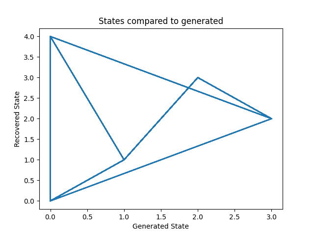
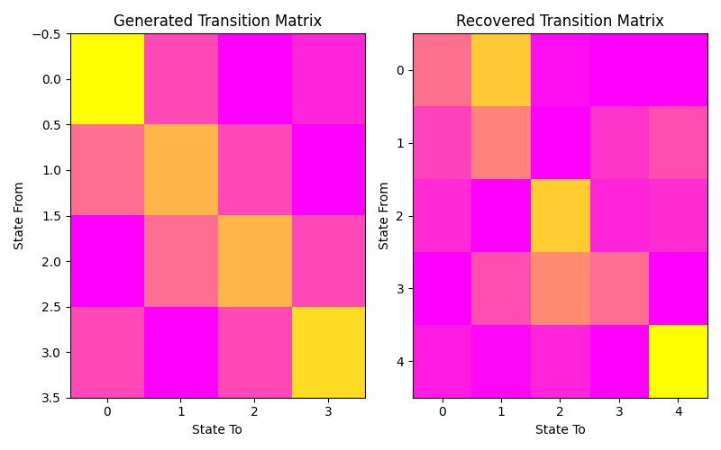
Let’s plot our states compared to those generated and our transition matrix to get a sense of our model. We can see that the recovered states follow the same path as the generated states, just with the identities of the states transposed (i.e. instead of following a square as in the first figure, the nodes are switch around but this does not change the basic pattern). The same is true for the transition matrix.

# plot model states over time
fig, ax = plt.subplots()
ax.plot(Z, states)
ax.set_title('States compared to generated')
ax.set_xlabel('Generated State')
ax.set_ylabel('Recovered State')
fig.show()

# plot the transition matrix
fig, (ax1, ax2) = plt.subplots(1, 2, figsize=(8, 5))
ax1.imshow(gen_model.transmat_, aspect='auto', cmap='spring')
ax1.set_title('Generated Transition Matrix')
ax2.imshow(model.transmat_, aspect='auto', cmap='spring')
ax2.set_title('Recovered Transition Matrix')
for ax in (ax1, ax2):
    ax.set_xlabel('State To')
    ax.set_ylabel('State From')

fig.tight_layout()
fig.show()

• 
•