Gaussian HMM of stock data
This script shows how to use Gaussian HMM on stock price data from
Yahoo! finance. For more information on how to visualize stock prices
with matplotlib, please refer to date_demo1.py of matplotlib.
from __future__ import print_function

import datetime

import numpy as np
from matplotlib import cm, pyplot as plt
from matplotlib.dates import YearLocator, MonthLocator
try:
    from matplotlib.finance import quotes_historical_yahoo_ochl
except ImportError:
    # For Matplotlib prior to 1.5.
    from matplotlib.finance import (
        quotes_historical_yahoo as quotes_historical_yahoo_ochl
    )

from hmmlearn.hmm import GaussianHMM


print(__doc__)
Get quotes from Yahoo! finance
quotes = quotes_historical_yahoo_ochl(
    "INTC", datetime.date(1995, 1, 1), datetime.date(2012, 1, 6))

# Unpack quotes
dates = np.array([q[0] for q in quotes], dtype=int)
close_v = np.array([q[2] for q in quotes])
volume = np.array([q[5] for q in quotes])[1:]

# Take diff of close value. Note that this makes
# ``len(diff) = len(close_t) - 1``, therefore, other quantities also
# need to be shifted by 1.
diff = np.diff(close_v)
dates = dates[1:]
close_v = close_v[1:]

# Pack diff and volume for training.
X = np.column_stack([diff, volume])
Run Gaussian HMM
print("fitting to HMM and decoding ...", end="")

# Make an HMM instance and execute fit
model = GaussianHMM(n_components=4, covariance_type="diag", n_iter=1000).fit(X)

# Predict the optimal sequence of internal hidden state
hidden_states = model.predict(X)

print("done")
Out:
fitting to HMM and decoding ...done
Print trained parameters and plot
print("Transition matrix")
print(model.transmat_)
print()
print("Means and vars of each hidden state")
for i in range(model.n_components):
print("{0}th hidden state".format(i))
print("mean = ", model.means_[i])
print("var = ", np.diag(model.covars_[i]))
print()
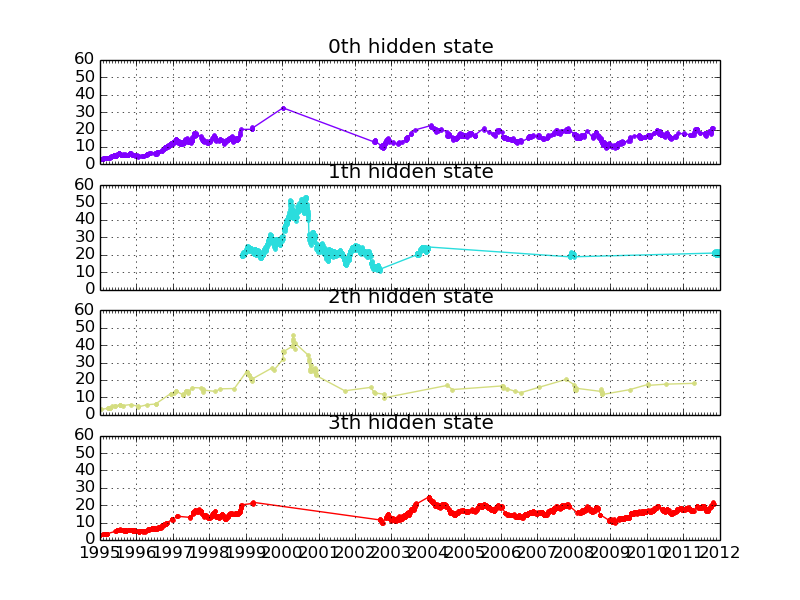
fig, axs = plt.subplots(model.n_components, sharex=True, sharey=True)
colours = cm.rainbow(np.linspace(0, 1, model.n_components))
for i, (ax, colour) in enumerate(zip(axs, colours)):
# Use fancy indexing to plot data in each state.
mask = hidden_states == i
ax.plot_date(dates[mask], close_v[mask], ".-", c=colour)
ax.set_title("{0}th hidden state".format(i))
# Format the ticks.
ax.xaxis.set_major_locator(YearLocator())
ax.xaxis.set_minor_locator(MonthLocator())
ax.grid(True)
plt.show()
Out:
  Transition matrix
[[  7.73505488e-01   1.21602143e-12   4.13525763e-02   1.85141936e-01]
 [  3.55338066e-15   9.79217702e-01   1.80611963e-02   2.72110180e-03]
 [  4.20116465e-01   1.18928463e-01   4.60955072e-01   1.91329669e-18]
 [  1.12652335e-01   3.25253603e-03   6.90794632e-04   8.83404334e-01]]

Means and vars of each hidden state
0th hidden state
mean =  [  2.19283455e-02   8.82098779e+07]
var =  [  1.26266869e-01   5.64899722e+14]

1th hidden state
mean =  [  2.40689227e-02   4.97390967e+07]
var =  [  7.42026137e-01   2.49469027e+14]

2th hidden state
mean =  [ -3.64907452e-01   1.53097324e+08]
var =  [  2.72118688e+00   5.88892979e+15]

3th hidden state
mean =  [  7.93313395e-03   5.43199848e+07]
var =  [  5.34313422e-02   1.54645172e+14]
Total running time of the script: (0 minutes 2.219 seconds)
Download Python source code:
plot_hmm_stock_analysis.py
Download IPython notebook:
plot_hmm_stock_analysis.ipynb