Sampling from and decoding an HMM

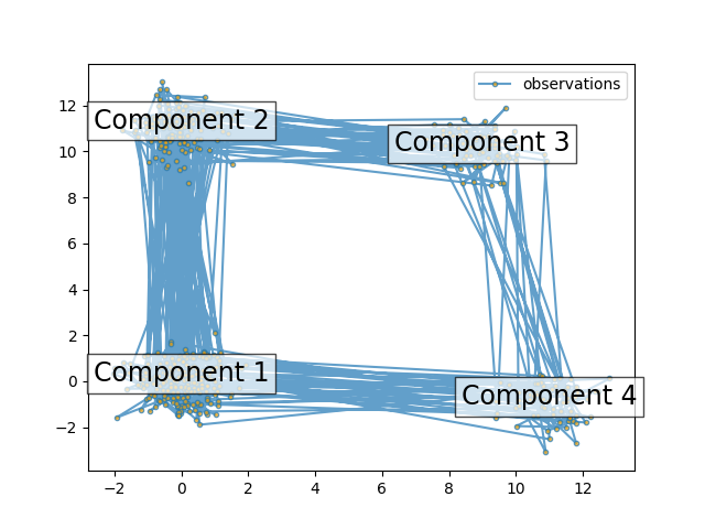
This script shows how to sample points from a Hidden Markov Model (HMM): we use a 4-state model with specified mean and covariance.

The plot shows the sequence of observations generated with the transitions between them. We can see that, as specified by our transition matrix, there are no transition between component 1 and 3.

Then, we decode our model to recover the input parameters.

import numpy as np
import matplotlib.pyplot as plt

from hmmlearn import hmm

# Prepare parameters for a 4-components HMM
# Initial population probability
startprob = np.array([0.6, 0.3, 0.1, 0.0])
# The transition matrix, note that there are no transitions possible
# between component 1 and 3
transmat = np.array([[0.7, 0.2, 0.0, 0.1],
                     [0.3, 0.5, 0.2, 0.0],
                     [0.0, 0.3, 0.5, 0.2],
                     [0.2, 0.0, 0.2, 0.6]])
# The means of each component
means = np.array([[0.0, 0.0],
                  [0.0, 11.0],
                  [9.0, 10.0],
                  [11.0, -1.0]])
# The covariance of each component
covars = .5 * np.tile(np.identity(2), (4, 1, 1))

# Build an HMM instance and set parameters
gen_model = hmm.GaussianHMM(n_components=4, covariance_type="full")

# Instead of fitting it from the data, we directly set the estimated
# parameters, the means and covariance of the components
gen_model.startprob_ = startprob
gen_model.transmat_ = transmat
gen_model.means_ = means
gen_model.covars_ = covars

# Generate samples
X, Z = gen_model.sample(500)

# Plot the sampled data
fig, ax = plt.subplots()
ax.plot(X[:, 0], X[:, 1], ".-", label="observations", ms=6,
        mfc="orange", alpha=0.7)

# Indicate the component numbers
for i, m in enumerate(means):
    ax.text(m[0], m[1], 'Component %i' % (i + 1),
            size=17, horizontalalignment='center',
            bbox=dict(alpha=.7, facecolor='w'))
ax.legend(loc='best')
fig.show()

Now, let’s ensure we can recover our parameters.

scores = list()
models = list()
for n_components in (3, 4, 5):
    for idx in range(10):
        # define our hidden Markov model
        model = hmm.GaussianHMM(n_components=n_components,
                                covariance_type='full',
                                random_state=idx)
        model.fit(X[:X.shape[0] // 2])  # 50/50 train/validate
        models.append(model)
        scores.append(model.score(X[X.shape[0] // 2:]))
        print(f'Converged: {model.monitor_.converged}'
              f'\tScore: {scores[-1]}')

# get the best model
model = models[np.argmax(scores)]
n_states = model.n_components
print(f'The best model had a score of {max(scores)} and {n_states} '
      'states')

# use the Viterbi algorithm to predict the most likely sequence of states
# given the model
states = model.predict(X)

Converged: True Score: -1573.7108963386934
Converged: True Score: -1197.7996923144096
Converged: True Score: -1099.3461183027766
Converged: True Score: -1099.346118302779
Converged: True Score: -1197.0500589957308
Converged: True Score: -1099.3461183027787
Converged: True Score: -1099.346118302777
Converged: True Score: -1099.3461183027746
Converged: True Score: -1099.3461183027773
Converged: True Score: -1099.3461183027785
Converged: True Score: -1099.896481015185
Converged: True Score: -1116.0565343040873
Converged: True Score: -934.6330821045342
Converged: True Score: -1018.3698546244416
Converged: True Score: -934.633082104536
Converged: True Score: -1113.59230593894
Converged: True Score: -900.5351999694603
Converged: True Score: -934.6330821045331
Converged: True Score: -934.6330821045333
Converged: True Score: -934.6330821045351
Converged: True Score: -1097.414913011789
Converged: True Score: -949.9904637505568
Converged: True Score: -1043.472609655898
Converged: True Score: -1088.5862030988894
Converged: True Score: -948.6103444099596
Converged: True Score: -1093.387922147961
Converged: True Score: -937.4606460228206
Converged: True Score: -976.1722394039717
Converged: True Score: -922.6262433609994
Converged: True Score: -959.3507610293523
The best model had a score of -900.5351999694603 and 4 states

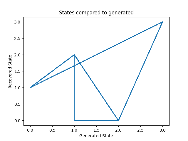
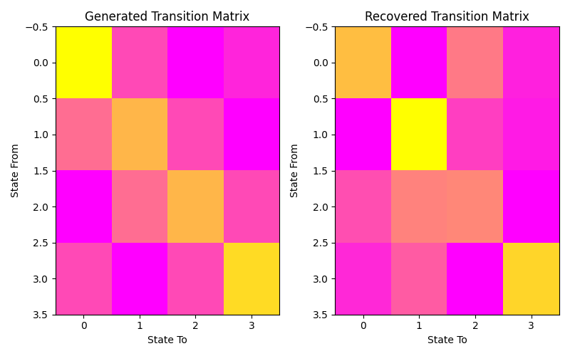
Let’s plot our states compared to those generated and our transition matrix to get a sense of our model. We can see that the recovered states follow the same path as the generated states, just with the identities of the states transposed (i.e. instead of following a square as in the first figure, the nodes are switch around but this does not change the basic pattern). The same is true for the transition matrix.

# plot model states over time
fig, ax = plt.subplots()
ax.plot(Z, states)
ax.set_title('States compared to generated')
ax.set_xlabel('Generated State')
ax.set_ylabel('Recovered State')
fig.show()

# plot the transition matrix
fig, (ax1, ax2) = plt.subplots(1, 2, figsize=(8, 5))
ax1.imshow(gen_model.transmat_, aspect='auto', cmap='spring')
ax1.set_title('Generated Transition Matrix')
ax2.imshow(model.transmat_, aspect='auto', cmap='spring')
ax2.set_title('Recovered Transition Matrix')
for ax in (ax1, ax2):
    ax.set_xlabel('State To')
    ax.set_ylabel('State From')

fig.tight_layout()
fig.show()

• 
•